
Predictability in physics versus AI/ML
Is predictability different? Maybe.

If you were ever home sick from school as an American child you have likely watched the television program, The Price is Right. The Price is Right is an American television show where contestants compete with each other by predicting the price of an item that is presented to them on stage. There are typically four contestants who are presented one item on stage. These contestants are expected to “predict” the correct price of items to within one cent. If they predict higher than the true value, they lose. If they predict less but someone predicts closer to the true price, they lose. If they win, they get to go on stage with Bob Barker (and later Drew Carey), who is a famous American person who is essentially only famous for doing this show. The contestant is then asked to play games all based on predicting the price of various items. As the contestant continues their success the items become more fabulous going from household items like a kitchen mop or some cleaning fluid, to cars, boats, or trips to Europe. The show has run regularly since 1972 for 52 seasons has over 10,000 episodes (here is a random one from 1995). Clearly, prediction is important to American society.
 - BoomerFlix.com - Classic ...")
Prediction and Predictability is, in essence, how much of a system can you describe from one state to the next. There are many different types of “predictable” systems and there are many different ways to characterize how to predict various systems. In The Price is Right, contestants try to “predict” the price of an item because they are making an educated guess of the cost of the item. The average person has purchased dish washing soap and likely can guess the price based on that experience. Many random systems have interesting conclusions when physically simulated. For example, fair coins have been demonstrated both in simulation and in observation to be biased to land on the side they started from. However, the key component across all systems is that if they are predictable, in some way, then we can summarize or compress some information about those systems in such a way that we can use that summarization to inform the evolution of the system in both cases that evolution is random or deterministic.
However, there are important differences in how statisticians and machine learning researchers define “predictability” versus how physicists define “predictability”. And thus, we are left with the question, “What is a prediction?” Below I will articulate two views: the machine learning view of prediction and the physicist view of prediction. There are more (e.g., I skip over Bayesians) but hopefully this is an interesting way to think about things. I focus on two key descriptive parameters, the R2 score which is common in machine learning regression tasks. And the Lyapunov exponent which is commonly used to examine chaotic regimes in various physical systems.
Statistics/ML view
Statisticians and machine learning people typically assume that there is a certain amount of “variance” in a system that can be explained by attempting to “linearize” the system of study. Variance is defined as:
This equation simply states that we want to know how far the “average” data point x is from the data average xbar. You often see in papers that use machine learning articulate their models using a similar equation called the R2 score:
If you compare the first and second equation the second equation is a ratio where we have replaced xhat with xbar. That simply means we compare how far does the data x deviate from the “model” xhat and it’s ratio to how far does the data x deviate from the average data value xbar (i.e., the previous equation). This R^2 value can have a maximum value of 1 and a minimum value of negative infinite, that is a model can be arbitrarily bad at predicting things. There are other statistics such as the root mean squared error, but they mostly attempt to articulate a particular view: how well does the statistical model capture the “predictability” of the system by how much variance is described by the statistical model? By adding more constraints, for example, keeping a validation data set separate from the training, you can extend the argument a bit and suggest your model is “generalizable” since it has operated successfully on data that it has never seen.

So far, the model xhat could be anything. We could articulate a model that says “if it rained yesterday p millimeters, today it will rain 2p millimeters.” And so if we have some rain data from a location we would first calculate our model output per day using the previous day’s precipitation and then use our R^2 equation to decide if we did a good job or not in predicting tomorrow’s precipitation. However, we could also use other data, e.g., the atmospheric pressure, as controlling parameters for tomorrow’s precipitation. As we add data variables to our model and it becomes more and more complex, we may want an algorithmic way to arrive at some optimum functional approximation to provide the prediction (e.g., a neural network or a gradient boosted machine or even a simple linear regression), but this is beyond the scope of this substack post. The point here is that from this framework, a system is considered “predictable” if we can somehow summarize the next state of the system by estimating how much variance is captured when we apply some model xhat.
Physicist view

Whereas the statistician's view of predictability assumes that there is some variance explained function to minimize, the physicist instead takes the view that dynamic systems either are deterministic or stochastic. Deterministic systems can be predicted into the future with some error that applies for when they diverge from prediction, and this can be due to chaos or simply the precision of the measurements. Stochastic systems are assumed to operate under some probability density function that is predictive of the overall behavior of the system but each individual event is random (e.g., nuclear decay rates). I will focus some on deterministic chaos but bear with me as of course I am not an expert on everything.
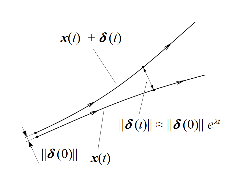
Chaos is defined as a system where the initial conditions can vastly affect the outcome. We can quantify this quite plainly with a Lyapunov exponent. The Lyapunov exponent attempts to measure the divergence between trajectories. If we examine the equation in the figure we can see there are two trajectories with some separation between them labeled x(t)+delta(t). This separation distance delta(t) can be described by the exponential equation, and when the exponent is positive we can see that the distance between the two trajectories will grow exponentially. This value is known as the Lyapunov exponent and is a common way to determine how quickly system trajectories will diverge from each other given various initial conditions. Of course, not all physics is chaotic, much of it is not (thankfully). In the non-chaotic cases we simply divert to the expectation that our physical laws are able to capture the trajectories of the system as time goes to infinity. That is, that the largest Lyapunov exponent is always valued at less than 0 is always true.
Discussion
Why is this important? It helps us, in a very general sense, determine when a system stops being predictable. However, let us now contrast the Lyapunov exponent, which is in some ways a measurement of similarity between trajectories of a system, to an R^2 score, which is also, essentially, a measurement of similarity between a model output and the naive assumption. In the R^2 score case, we are measuring the similarity of our machine learning model xhat to the naive model xbar. When this similarity is poor (i.e., R^2 is approaching 1.0), we typically claim that our model arrives at a good understanding of the system because we assume that this increase in R^2 value is because there is a decrease in unexplainable variance (or perhaps randomness). We compare different machine learning models with different features (i.e., variables or data) hoping that by adding more context to the model with additional information, we will be able to build a model that maximizes the R^2 score. This can of course be misused or misattributed and problems like “p-hacking”, violating model assumptions, unexplained heteroskedasticity, and other issues that I won’t go into here.
In the Lyapunov exponent case, we are saying something different. We are not concerned with what data we should add into our model, we typically have a pre-specified model. We assume that we have generated a relationship (e.g., through phase space reconstruction) that explains how different parts of the system interact. When the Lyapunov exponent becomes positive, the trajectories diverge from each other and can no longer be predicted except through our knowledge of the system initial conditions. No minimization of variance in the system matters, no additional variables or data concerning the system matters, we simply cannot predict chaos.
However, you may have read about recent work, such as reservoir models, NBEATS, mamba, etc., which claims to predict such chaotic systems to some degree past the point where Lyapunov exponents become positive. Taken at face value, this is profound. But why is this true?
Personally, I don’t actually know the answer to this question and feel like it is an open question. Perhaps other people know the answer to this question. Perhaps they might find it trivial. In any case, I will suggest, is a good time to stop and ask you to watch a few talks from the AI conference that I helped organize in October 2024 where I address this. I would suggest watching the talks by William Gilpin and Anders Malthe-Sørenssen. William’s talk directly dives into the predictability issue. Anders' talk is a discussion about understanding how a very complex generative machine learning model arrives at its solution. I think these talks begin to unravel why this is true, but the truth is we simply do not know. Or at least, I don’t know.

This was originally written as an internal newsletter which I have expanded and re-edited for here.